Random Variable of the Continuous Type

A continuous random variable has two main characteristics:

1. the set of its possible values is uncountable;

2. we compute the probability that its value will belong to a given interval by integrating a function called probability density function.

On this page we provide a definition of continuous variable, we explain it in great detail, we provide several examples and we derive some interesting properties.

Table of contents

1. Definition

2. Dealing with integrals

3. Probabilities are assigned to intervals

4. Examples

   1. Example 1

   2. Example 2

5. Cumulative distribution function

6. All the realizations have zero probability

7. The support is uncountable

8. Continuous vs discrete

9. Understanding the definition

   1. Exploring inconvenient alternatives - Enumeration of the possible values

   2. Exploring inconvenient alternatives - All the rational numbers

   3. A more convenient alternative - Intervals of real numbers

10. Other explanations

11. Expected value

12. Higher moments and functions

13. Variance

14. Conditional expectation

15. Common continuous distributions

16. Synonyms

17. More details

18. Keep reading the glossary

Here is a formal definition.

Definition A random variable is said to be continuous if and only if the probability that it will belong to an interval can be expressed as an integral: where the integrand function is called the probability density function of .

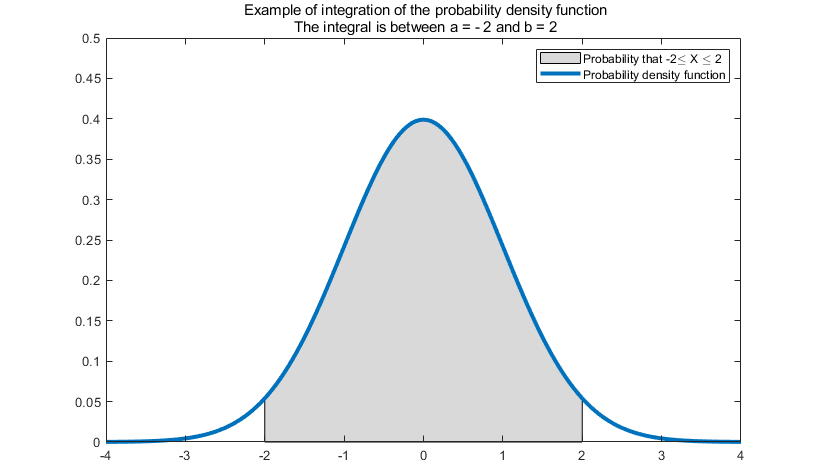
If you are not familiar with integrals, you can read the lecture on the basics of integration.

It is anyway important to remember that an integral is used to compute an area under a curve.

In the definition of a continuous variable, the integral is the area under the probability density function in the interval between and .

The first thing to note in the definition above is that the distribution of a continuous variable is characterized by assigning probabilities to intervals of numbers.

Contrast this with the fact that the distribution of a discrete variable is characterized by assigning probabilities to single numbers.

Before explaining why the distribution of a continuos variable is assigned by intervals, we make some examples and discuss some of its mathematical properties.

Here are some examples.

Example 1

Let be a continuous random variable that can take any value in the interval .

Let its probability density function be

Then, for example, the probability that takes a value between and can be computed as follows:

Example 2

Let be a continuous random variable that can take any value in the interval with probability density function

The probability that the realization of will belong to the interval is

As a consequence of the definition above, the cumulative distribution function of a continuous variable is

The derivative of an integral with respect to its upper bound of integration is equal to the integrand function. Therefore,

In other words, the probability density function is the derivative of the cumulative distribution function .

Any single realization has zero probability of being observed because

Therefore, in a continuous setting zero-probability events are not events that never happen. In fact, they do happen all the time: all the possible values have zero probability, but one of them must be the realized value.

This property, which may seem paradoxical, is discussed in the lecture on zero-probability events.

Another consequence of the definition given above is that the support of a continuous random variable must be uncountable.

In fact, by the previous property, if the support (the set of values the variable can take) was countable, then we would have which is a contradiction because the probability that a random variable takes at least one of all its possible values must be 1.

In order to sharpen our understanding of continuous variables, let us highlight the main differences with respect to discrete variables found so far.

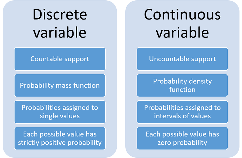
The main characteristics of a discrete variable are:

• the set of values it can take (so-called support) is countable;

• its probability distribution is described by a probability mass function that assigns a probability to each single value in the support;

• the values belonging to the support have a strictly positive probability of being observed.

By contrast, the main characteristics of a continuous random variable are:

• the set of values it can take is uncountable;

• its probability distribution is described by a probability density function that assigns probabilities to intervals of values;

• each value belonging to the support has zero probability of being observed.

Why do we define a mathematical object that has such a counterintuitive property (all possible values have zero probability)?

The short answer is that we do it for mathematical convenience.

Suppose that we are trying to model a certain variable that we see as random, for example, the proportion of atoms that exhibit a certain behavior in a physics experiment.

In general, a proportion is a number in the interval .

Exploring inconvenient alternatives - Enumeration of the possible values

If we knew exactly the total number of atoms involved in the experiment, then we would also know that the proportion could take the values

However, in many cases the exact number of atoms involved in an experiment is not only huge, but also not known precisely.

What do we do in such cases? Can we enumerate all the possible values of ?

Theoretically, we could write down the list in (1) for every value of that we deem possible and then take the union of all the lists.

The resulting union would be a finite support for our random variable , to which we would then need to assign probabilities.

Given that the possible values of are likely in the trillions, such an approach would be highly impractical.

Exploring inconvenient alternatives - All the rational numbers

An alternative is to consider the set of all rational numbers belonging to the interval .

Remember that a rational number is the ratio of two integers. As a consequence, the set of rational numbers in includes all the possible values of the proportion . Moreover, it is a countable set.

Thus, we can use a probability mass function to assign probabilities to it, without resorting to exotic density functions.

Unfortunately, this approach works only in special cases.

For example, suppose that all the possible values of are deemed to be equally likely. There is no way to assign equal probabilities to all the values in the set of rational numbers in because it contains infinitely many numbers (the probability of a single number should be , which does not work).

A more convenient alternative - Intervals of real numbers

The third alternative is provided by continuous random variables.

We can consider the whole interval of real numbers and assign probabilities to its sub-intervals using a probability density function.

In the case in which all the values are deemed equally likely, we use a constant probability density function, equal to on the whole interval (called a uniform distribution).

This brilliantly solves the problem, although we need to accept the fact that the question "What is the probability that will take a specific value ?" does not make much sense any longer.

The questions that we can still ask are of the kind "What is the probability that will take a value close to ?" provided that we define precisely what we mean by close in terms of an interval (e.g., where is an accuracy parameter that we define).

You can find other explanations and examples that help to understand the definition of continuous variable in:

• this blog post on Math Insight;

• these lecture notes used in the Mathematics Department of the University of Colorado Boulder;

• our page on the probability density function.

The expected value of a continuous random variable is calculated as

See the lecture on the expected value for explanations and examples.

The moments of a continuous variable can be computed as and the expected value of a transformation is

The variance can be computed by first calculating moments as above and then using the variance formula

The conditional expected value of a continuous random variable can be calculated using its conditional density function (see the lecture on conditional expectation for details and examples).

The next table contains some examples of continuous distributions that are frequently encountered in probability theory and statistics.

Name of the continuous distribution	Support
Uniform	All the real numbers in the interval [0,1]
Normal	The whole set of real numbers
Chi-square	The set of all non-negative real numbers

Continuous random variables are sometimes also called absolutely continuous.

Continuous random variables are discussed also in:

• the lecture on random variables;

• the glossary entry on the probability density function.

Multivariate generalizations of the concept are presented here:

• continuous random vector;

• random matrix.

Next entry: Absolutely continuous random vector

Please cite as:

Taboga, Marco (2021). "Continuous random variable", Lectures on probability theory and mathematical statistics. Kindle Direct Publishing. Online appendix. https://www.statlect.com/glossary/absolutely-continuous-random-variable.

weaveracloned.blogspot.com

Source: https://www.statlect.com/glossary/absolutely-continuous-random-variable

Share this post